Research and Analysis of Coal Volatile Matter and Calorific Value Based on Laser-Induced Breakdown Spectroscopy
published: 18 July 2025 | https://doi.org/10.63174/xdi.SOBF9341
Abstract
Laser-induced breakdown spectroscopy (LIBS) technology has demonstrated significant application value in coal industrial process monitoring due to its advantages of rapid, in-situ, and multi-element synchronous detection. This study systematically investigates a rapid detection method for coal volatile matter and calorific value based on LIBS technology, addressing the issues of low efficiency and time-consuming processes associated with traditional coal quality analysis methods. Conventional methods for selecting characteristic spectral lines from coal samples are time-consuming and exhibit poor accuracy. Therefore, this study employs variable importance in projection (VIP) to screen key variables in coal samples. The research utilized 84 coal samples. Firstly, a full-spectrum analysis model for volatile matter and calorific value was established based on partial least squares regression (PLSR). The coefficients of determination (R²) for the training and test sets of volatile matter and calorific value were 0.9610 and 0.9485, and 0.8972 and 0.9312, respectively. The root-mean-square error of cross-validation (RMSECV) and the root-mean-square error of prediction (RMSEP) were 0.3678 % and 0.5204 %, and 0.2999 MJ/kg and 0.2515 MJ/kg, respectively. Subsequently, VIP variable screening was applied for PLSR modeling, resulting in improved R² values of 0.9773 and 0.9569, and 0.9263 and 0.9348, respectively. The RMSECV and RMSEP decreased to 0.2804 % and 0.4759 %, and 0.2538 MJ/kg and 0.2450 MJ/kg, respectively. This research results indicate that the established analytical framework can be extended to other solid fuel quality detection fields, playing a significant role in achieving intelligent monitoring of industrial processes.
1. Introduction
Laser-Induced Breakdown Spectroscopy (LIBS) is an analytical technique based on atomic emission spectroscopy that enables both qualitative and quantitative elemental analysis. It works by analyzing the characteristic emission spectral lines generated during plasma evolution to determine the content of various elements in a sample [1]. Due to its advantages of rapid detection, non-destructive measurement, and the capability for online monitoring, LIBS has attracted growing attention in both industrial applications and scientific research. It holds broad application prospects in fields such as biomedicine [2]–[4], food safety [5]–[7], environmental protection [8]–[10], and archaeology [11]–[13]. In recent years, LIBS has also demonstrated significant potential in coal analysis. Coal is a critical component of the global energy structure. Its quality parameters—such as volatile matter and calorific value—directly influence combustion efficiency, pollutant emissions, and industrial performance [14]. Generally, coal with higher volatile content ignites more easily and burns more completely. However, excessive volatile matter may lead to instability and difficulty in controlling the combustion process. Calorific value, defined as the energy released by the complete combustion of a unit mass of coal, is one of the most important indicators for evaluating energy conversion efficiency. It significantly affects economic parameters such as boiler thermal efficiency and coal consumption in power generation. Traditional methods for coal composition analysis, including chemical and proximate analysis, suffer from several limitations. These include lengthy analysis times, destructive sampling, and complex procedures. As a result, they fall short of meeting the increasing demand for rapid and real-time detection in modern industrial environments. LIBS offers a viable alternative by using high-energy laser pulses to ablate the sample and generate plasma. The emitted light is then analyzed to determine the elemental composition. This enables correlations between spectral features and key coal quality indicators such as ash content, volatile matter, and calorific value. For example, Li et al. [15] proposed a method combining LIBS with X-ray fluorescence spectroscopy (XRF) to predict coal calorific value based on the relationship between elemental content and energy output. Using principal component analysis and multiple regression, they achieved a prediction RMSEP of 0.9 MJ/kg. Despite its advantages, LIBS-based coal detection still faces technical challenges. These include matrix effects, spectral interference, and limited accuracy in quantitative models. In particular, improving model optimization for volatile matter, ash content, and calorific value remains a key research direction. In this study, we established a LIBS-based analytical framework using 84 coal samples collected from thermal power plants. After sample preparation, data acquisition, and preprocessing, we developed quantitative models using the Partial Least Squares Regression (PLSR) algorithm combined with Variable Importance in Projection (VIP) screening [16]. Initially, a full-spectrum PLSR model was built using 67 training samples [17], and the results were validated on a test set. Then, VIP screening was applied to reduce the feature space by 52.54%, followed by re-modeling.
The experimental results demonstrate that VIP screening significantly enhances model fitting and prediction performance. For the test set, the coefficient of determination (R²) for volatile matter and calorific value increased from 0.9485 and 0.9312 to 0.9569 and 0.9348, respectively. Meanwhile, the RMSECV and RMSEP values showed notable decreases. These findings demonstrate that the proposed LIBS-based framework offers a promising approach for rapid and accurate coal quality assessment.
2. Experiment
2.1. LIBS experimental setup
The main hardware components of the LIBS experimental setup include: a Q-switched Nd: YAG pulsed laser, a multi-channel spectrometer, a half-wave plate, a polarizing beam splitter, mirrors, a focusing lens, a collection lens, a fiber optic probe, a multimode fiber transmission line, a laser energy meter, a three-dimensional motion platform, and a computer. The laser system operated with a pulse energy of 30-110 mJ, repetition frequency of 1-10 Hz, and spot size ≤10 mm, while the spectrometer covered a wavelength range of 181-770 nm with a resolution of 0.058-0.068 nm. A schematic diagram of the LIBS experimental system is shown in Figure 1.
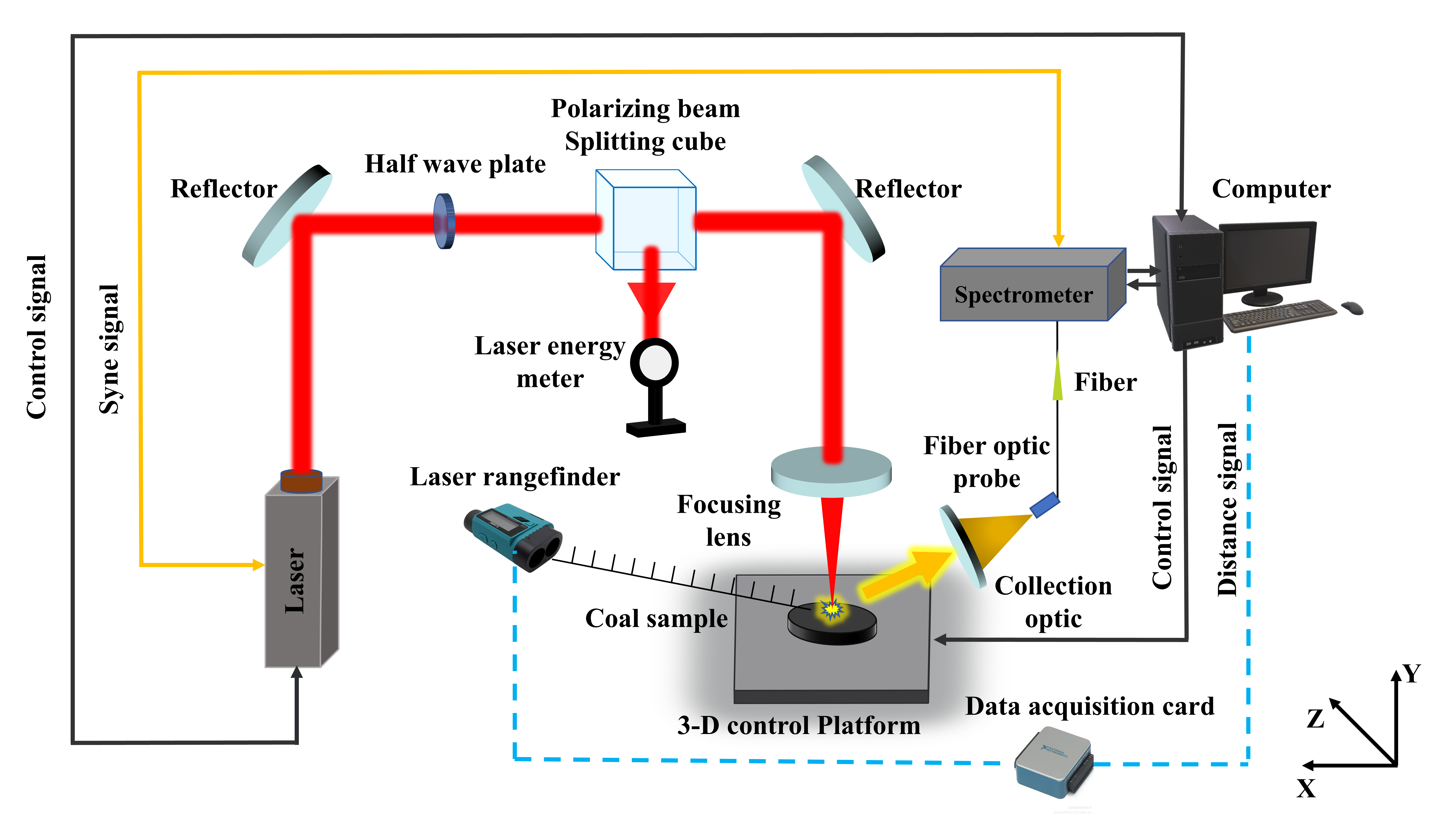
Figure 1. Schematic diagram of the LIBS experimental system.
The working procedure of the LIBS experimental system is as follows: A Q-switched Nd: YAG laser with a working wavelength of 1064 nm serves as the laser source, and its operating energy is determined using a half-wave plate and a polarizing beam splitter. The laser beam is then focused onto the surface of the coal sample under test by two mirrors and a focusing lens to induce plasma formation. The light emitted by plasma during its transition from excited states to lower energy levels or the ground state is collected by a lens and transmitted via a fiber optic probe and multimode fiber to the spectrometer, where the optical signals are converted into electrical signals and sent to a computer for analysis.
In Figure 1, a laser rangefinder measures the real-time focal distance of the sample through a data acquisition card, adjusting the focal position of the pulsed laser after passing through the focusing lens. The Z-axis of the three-dimensional motion platform receives signals from the laser rangefinder and provides positional feedback. Finally, the coal sample is placed on the three-dimensional motion platform for S-shaped scanning. The X- and Y-axes of the platform are controlled by the computer to perform a 5×5 grid laser ablation on the sample, with each sampling point subjected to 5 repeated laser pulses. In total, 125 × 4094 spectral data points are acquired per sample.
2.2. Experimental samples
The 84 coal samples used in this experiment were obtained from a thermal power plant. The preparation of coal samples for LIBS analysis was conducted as follows: First, the 84 coal samples were ground into powder with particle sizes below 0.2 mm and stored in individual sample bags. After drying, approximately 3.5 g of each sample was compressed into a pellet using a hydraulic press under 40-ton pressure for over 30 seconds. This process yielded coal pellets with a diameter of 35 mm, a thickness of approximately 5 mm, and a smooth surface. The prepared pellets were then sealed, labeled, and stored for subsequent LIBS experiments.
Figure 2 displays the R² values of PLSR models built using 30 samples and 67 samples, respectively. The comparison reveals that the model constructed with 67 samples performs better, as it accounts for approximately 80% of the total 84 samples (close to an 8:2 ratio), thereby mitigating the risks of underfitting and overfitting.
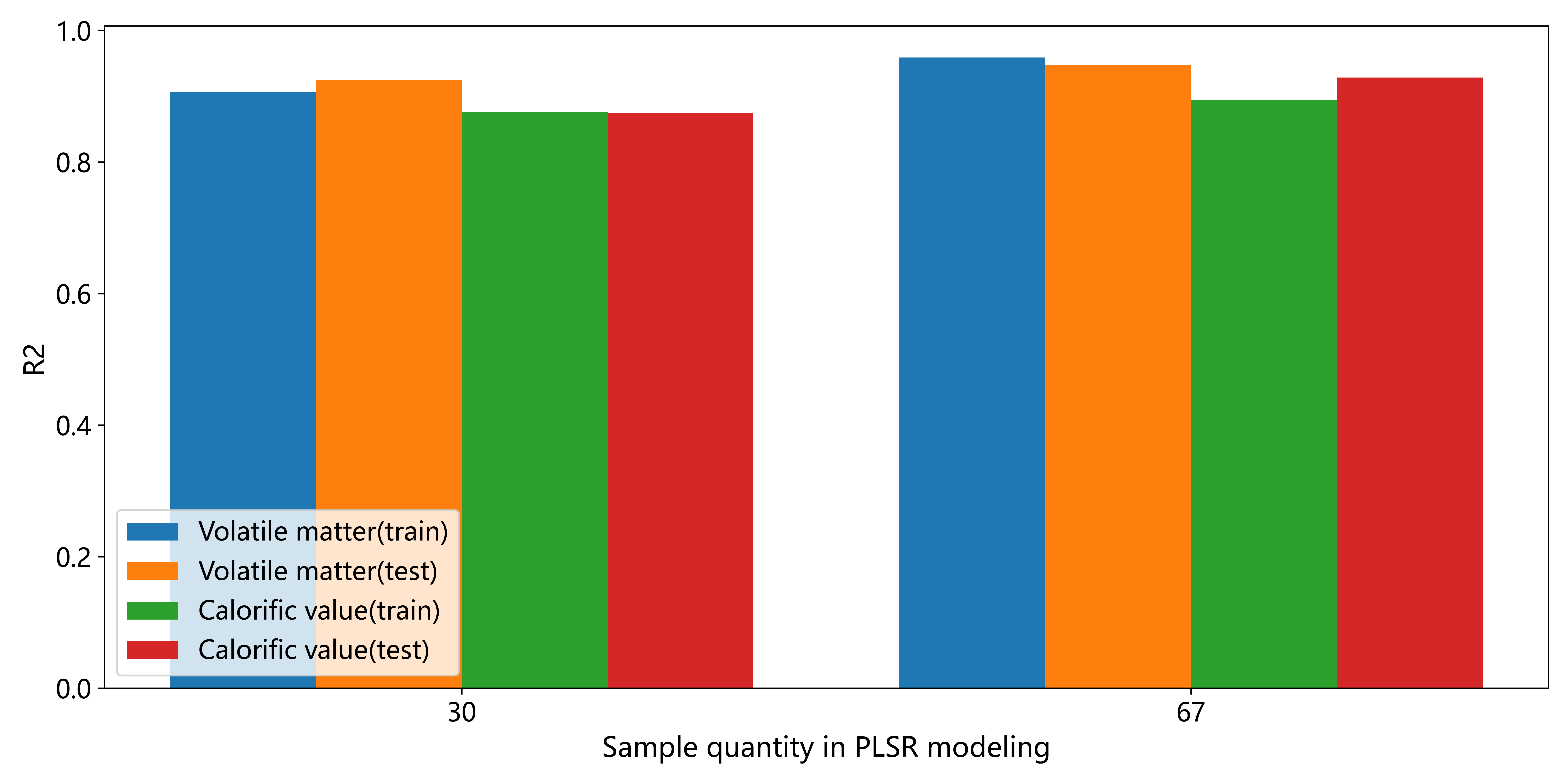
Figure 2. The comparison of R2 across different modeling samples.
Table 1 lists the specific sample numbers (1–84), volatile matter content (13.10 %–21.88 %), and reference calorific values (21.662–25.870 MJ/kg) of the 84 coal samples. Among these, 17 coal samples were randomly selected as the test set, while the remaining 67 samples served as the training set. The test set samples are explicitly marked in Table 1.
Table 1. Reference Values of Volatile Matter Content and Calorific Value for the 84 Samples
| NO. | Vad (%) (13.10 %–21.88 %) | Qad (MJ/kg) (21.662–25.870 MJ/kg) |
NO. | Vad (%) (13.10 %–21.88 %) | Qad (MJ/kg) (21.662–25.870 MJ/kg) |
||
|---|---|---|---|---|---|---|---|
| 1* | 16.84 | 24.796 | 43 | 20.38 | 23.900 | ||
| 2 | 16.40 | 24.990 | 44 | 20.37 | 24.130 | ||
| 3 | 16.50 | 25.080 | 45 | 19.29 | 23.410 | ||
| 4 | 16.66 | 25.580 | 46 | 15.38 | 23.336 | ||
| 5* | 16.41 | 24.590 | 47 | 16.52 | 23.484 | ||
| 6 | 15.40 | 24.380 | 48* | 18.03 | 23.950 | ||
| 7 | 15.84 | 24.800 | 49 | 16.62 | 25.230 | ||
| 8 | 14.73 | 24.490 | 50 | 17.02 | 24.620 | ||
| 9 | 16.10 | 23.070 | 51 | 15.88 | 24.820 | ||
| 10 | 16.38 | 23.530 | 52 | 14.68 | 23.330 | ||
| 11* | 14.72 | 24.000 | 53 | 15.97 | 24.290 | ||
| 12 | 13.98 | 22.444 | 54 | 17.08 | 24.300 | ||
| 13* | 16.17 | 23.070 | 55* | 16.16 | 23.200 | ||
| 14 | 17.06 | 23.358 | 56* | 14.72 | 22.760 | ||
| 15 | 15.22 | 21.700 | 57 | 15.12 | 23.290 | ||
| 16 | 17.57 | 23.360 | 58 | 16.30 | 21.908 | ||
| 17 | 16.08 | 22.946 | 59* | 14.80 | 21.662 | ||
| 18 | 17.95 | 23.940 | 60 | 15.40 | 22.703 | ||
| 19* | 19.94 | 24.470 | 61 | 16.22 | 22.200 | ||
| 20 | 16.34 | 24.270 | 62 | 17.88 | 22.650 | ||
| 21 | 16.26 | 23.620 | 63 | 16.06 | 23.186 | ||
| 22 | 15.26 | 23.690 | 64 | 16.78 | 24.070 | ||
| 23* | 13.16 | 23.824 | 65 | 20.90 | 24.460 | ||
| 24 | 16.29 | 24.150 | 66* | 15.87 | 24.100 | ||
| 25 | 15.13 | 23.580 | 67 | 14.88 | 22.730 | ||
| 26 | 13.92 | 23.630 | 68 | 14.98 | 23.373 | ||
| 27 | 15.68 | 23.500 | 69 | 14.72 | 23.630 | ||
| 28 | 15.12 | 24.310 | 70 | 13.10 | 22.720 | ||
| 29 | 14.38 | 24.650 | 71* | 13.29 | 23.190 | ||
| 30 | 16.30 | 24.830 | 72 | 14.88 | 23.290 | ||
| 31 | 17.02 | 24.360 | 73 | 15.76 | 24.320 | ||
| 32 | 15.00 | 23.610 | 74* | 16.72 | 23.770 | ||
| 33 | 15.19 | 25.720 | 75 | 15.45 | 23.970 | ||
| 34* | 16.64 | 25.870 | 76 | 15.48 | 22.790 | ||
| 35 | 14.21 | 24.590 | 77 | 16.20 | 23.370 | ||
| 36* | 21.81 | 25.040 | 78 | 15.62 | 24.100 | ||
| 37 | 21.62 | 25.780 | 79 | 16.05 | 23.100 | ||
| 38 | 21.88 | 25.520 | 80 | 15.58 | 21.990 | ||
| 39 | 18.97 | 25.010 | 81 | 19.71 | 24.090 | ||
| 40 | 19.34 | 24.930 | 82* | 18.50 | 23.530 | ||
| 41* | 19.99 | 24.710 | 83 | 15.28 | 24.890 | ||
| 42 | 20.05 | 24.870 | 84 | 16.60 | 23.070 | ||
The samples marked with * in the table represent the test set.
2.3. Preprocessing procedure
In practical applications of LIBS technology, raw spectral data often contain significant interference signals and random errors due to instrumental noise, environmental disturbances, plasma instability, and other factors. Therefore, spectral preprocessing is a critical step to ensure data reliability and model accuracy, and the spectral preprocessing procedure is illustrated in Figure 3.
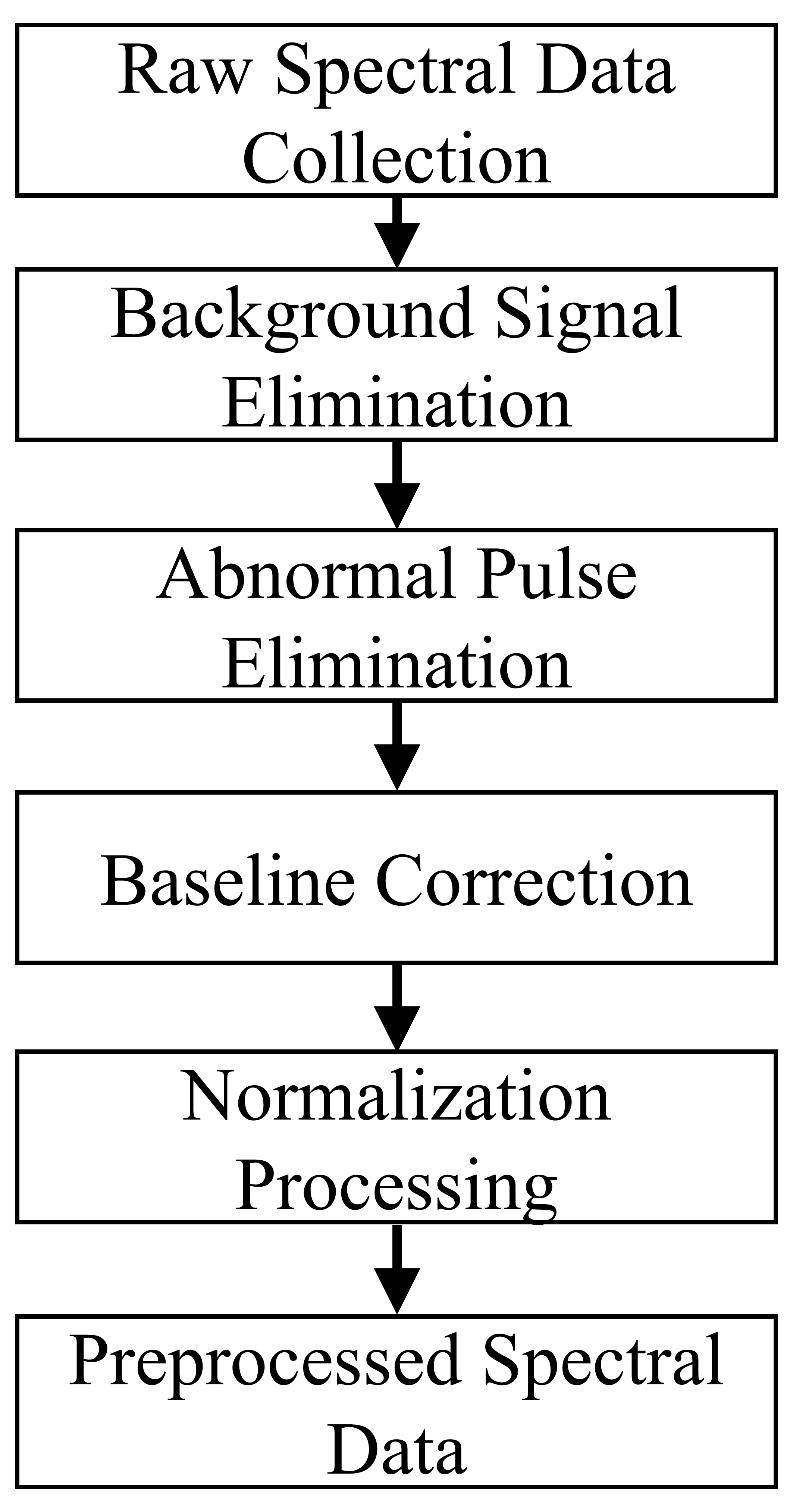
Figure 3. Spectral preprocessing pipeline.
The raw LIBS spectral data undergoes multistage processing to eliminate systematic noise and environmental interference. The specific workflow is as follows:
2.3.1 Background Signal Elimination
The dark current subtraction method was employed: Blank background spectra were first acquired as reference, then subtracted from each measured spectrum with negative values truncated.
I = Iraw − Ibackground (1)
In Equation (1), I represents the spectral intensity after background removal, Iraw denotes the originally acquired spectral intensity, and I background corresponds to the measured environmental background spectral intensity.
2.3.2 Abnormal Pulse Elimination
Hard threshold criterion: Directly eliminate spectra containing the detector saturation value of 65535.
Statistical criterion: Calculate the sum of squared deviations from the mean (SS) for each pulse, exclude abnormal pulses exceeding 1.1 times the mean value.
${SS}_{i} = \sum_{k = 1}^{n}\left( x_{i,k} - {\overline{x}}_{i} \right)^{2}$ (2)
In Equation (2), SSi: the sum of squared deviations from the mean for the i-th pulse; xi, k: the spectral intensity of the k-th data point in the i-th pulse; ${\overline{x}}_{i}$: the mean spectral intensity of the i-th pulse; n: the number of data points contained in a single pulse.
Elimination criterion: If SSi > 1.1 ×$\overline{SS}$, then the pulse is considered an outlier and should be eliminated. Here, $\overline{SS}$ represents the mean sum of squared deviations from the mean for all pulses.
2.3.3 Baseline Correction
A dynamic sliding window minimum subtraction method was applied:
A sliding window of 16 pixels (half-width of 8 pixels) was set to calculate the local minimum point-by-point as the estimated baseline. The baseline was then subtracted to obtain the net signal intensity.
Inet = I − B (3)
In Equation (3): Inet: The baseline-corrected net signal intensity. I: The spectral intensity before baseline correction.B: The baseline intensity estimated using a sliding window.
Calculation of baseline B: For each pixel j, within the window [j − 8, j + 8] (totaling 16 pixels), take the minimum spectral intensity Bj = min{Ij − 8, Ij − 7, ⋯, Ij + 8}.
2.3.4 Normalization Processing
Perform Min-Max normalization to eliminate the impact of energy fluctuations:
$I_{mapminmax} = \frac{I - I_{\min}}{I_{\max} - I_{\min}}$ (4)
In Equation (4), Imapminmax represents the normalized spectral intensity, I is the spectral intensity value of each dataset after baseline correction, Imin is the minimum spectral intensity in each dataset, and Imax is the maximum spectral intensity in each dataset.
In Figure 4, Figure 4(a) shows the original spectral curve of Coal Sample No. 5, while Figure 4(b) displays the spectral curve of the same sample after preprocessing. By comparison, it can be observed that the relative intensity of the preprocessed spectrum differs from that of the original spectrum. This is because preprocessing significantly removes noise and irrelevant information from the spectral data. Additionally, the normalization process provides reliable spectral data for modeling various indicators of coal samples, facilitating model processing.
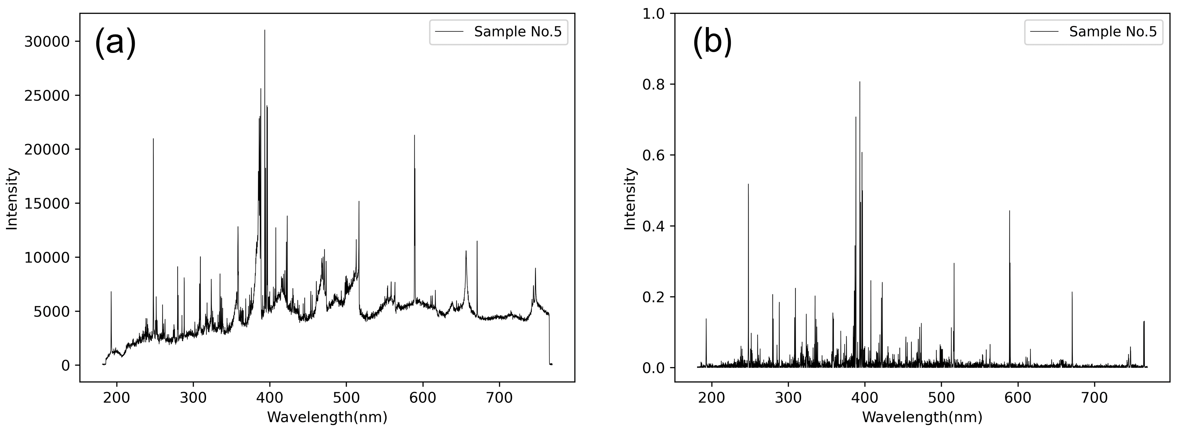
Figure 4. (a) Original spectrum (b) Preprocessed spectrum (Coal Sample No. 5).
2.4. Model Evaluation Metrics
In Equation (5), R² represents the goodness of fit between calculated (predicted) values and actual values. The closer R² is to 1, the better the model's fitting performance. Equations (6) RMSECV and (7) RMSEP are used to evaluate the differences between leave-one-out cross-validation values, predicted values and actual values. Smaller values indicate more accurate predictions.
$R^{2} = 1 - \frac{\sum_{i}^{n}\left( y_{i} - {\widehat{y}}_{i} \right)^{2}}{\sum_{i}^{n}\left( y_{i} - {\overline{y}}_{i} \right)^{2}}$ (5)
$RMSEP = \sqrt{\frac{\sum_{i}^{m}\left( y_{i} - {\widehat{y}}_{i} \right)^{2}}{m}}$ (6)
$RMSECV = \sqrt{\frac{\sum_{i}^{n}\left( y_{i} - {\widehat{y}}_{i} \right)^{2}}{n - 1}}$ (7)
In the equation (5) - (7), yi and ŷi represent the reference value and predicted value of coal component content respectively, while ${\overline{y}}_{i}$ denotes the average reference value of coal component content. Here, n and m indicate the number of coal samples in the training set and test set respectively.
2.5. Model establishment and parameter selection
This experiment used 67 coal samples as the training set and the remaining 17 samples as the test set. First, a PLSR model without VIP variable screening was established, developing full-spectrum PLSR quantitative regression models for volatile matter and calorific value using the training set samples. The latent variables (LVs) for the volatile matter and calorific value PLSR models were then selected using leave-one-out cross-validation, with RMSE serving as the evaluation metric. Figure 5 shows the RMSE under different numbers of latent variables: (a) LV selection for volatile matter PLSR and (b) LV selection for calorific value PLSR.As the number of latent variables increased, RMSE initially decreased rapidly because the first few LVs captured the strongest covariance relationships (i.e., primary signals) in the data, significantly enhancing the model's explanatory power for the response variables. Subsequently, the rate of RMSE reduction slowed and gradually stabilized, as later LVs contained only weak signals or noise, contributing marginally to model improvement. At this stage, the marginal benefit of adding more LVs for error reduction diminished. Since calorific value required more LVs (8) to capture complex relationships compared to volatile matter (which needed only 6), a compromise of 7 LVs was selected to balance the performance of both models. After determining the optimal number of LVs, the PLSR quantitative regression model was rebuilt using this optimal LV count, and predictions were made on the test set samples. Finally, VIP screening was applied with a threshold of 0.9. Following preprocessing, the full spectrum underwent variable selection, reducing the number of dependent variable features by 52.54 %. Subsequently, PLSR modeling and analysis were performed again.
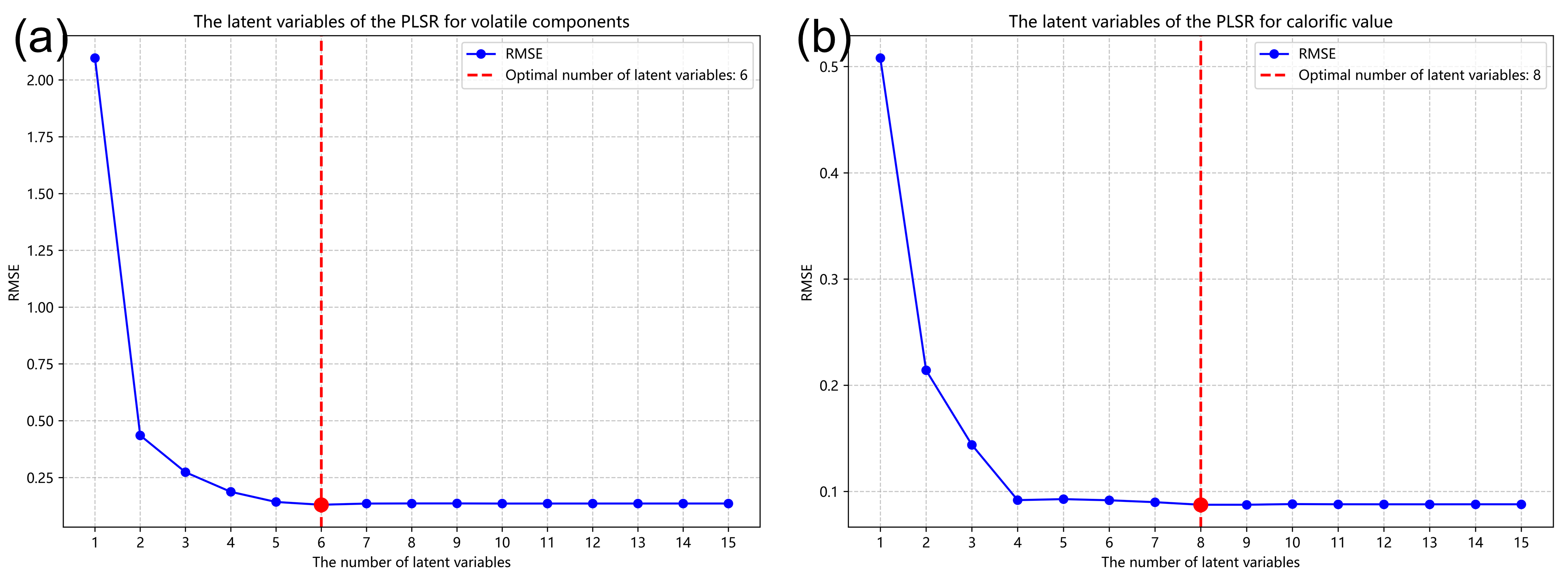
Figure 5. (a) LV selection for volatile matter PLSR (b) LV selection for calorific value PLSR.
3. Results and discussion
3.1. PLSR
The final PLSR results for volatile matter and calorific value are presented in Figure 6(a) and Figure 6(b), with blue dots denoting the training set, red dots the test set, and the red dashed line representing the linear fit between leave-one-out cross-validation values and true values. For volatile matter, the training set R² was 0.9610, test set R² 0.9485, RMSECV 0.3678 %, and RMSEP 0.5204 %. The corresponding parameters for calorific value were 0.8972 (training set R²), 0.9312 (test set R²), 0.2999 MJ/kg (RMSECV), and 0.2515 MJ/kg (RMSEP).
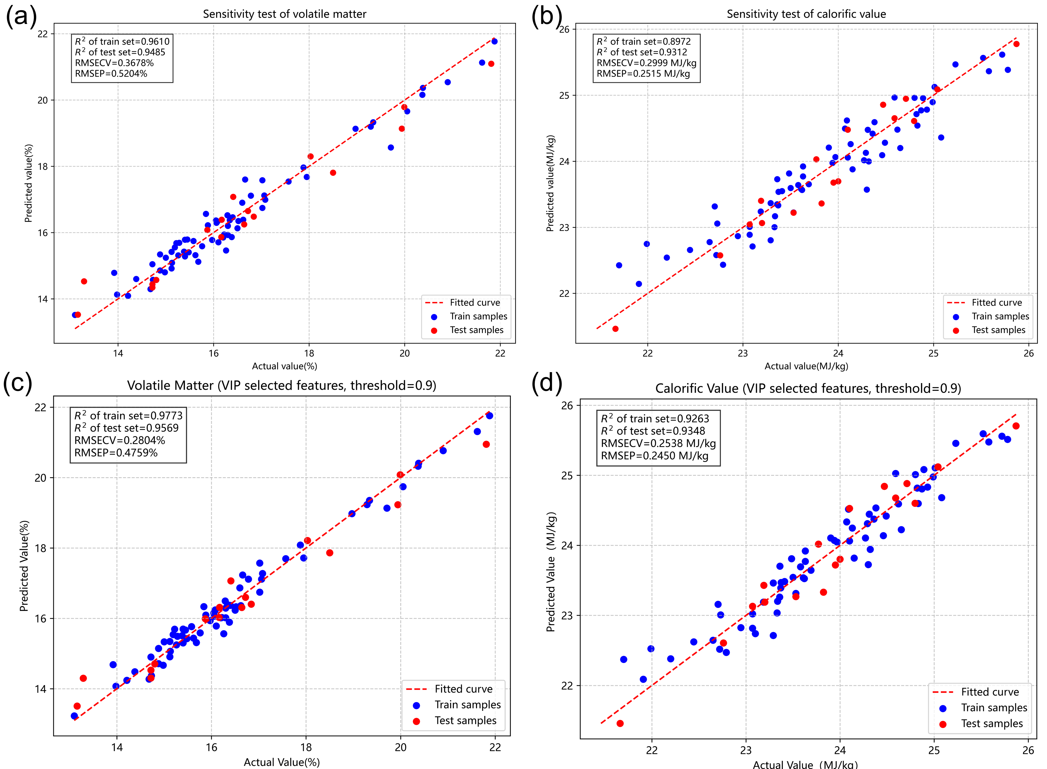
Figure 6. (a) Volatile matter PLSR (b) Calorific value PLSR (c) Volatile matter PLSR+VIP (d) Calorific value PLSR+VIP.
3.2. VIP Screening + PLSR
Table 2 displays the R2 values of the test-set under different VIP screening thresholds. Through comparison and comprehensive consideration, the best performance is achieved when the threshold is set at 0.9. Figure 6 (c) and Figure 6 (d) show the modeling results combining VIP screening with PLSR. After VIP variable selection, the training and test set R² values for volatile matter increased to 0.9773 and 0.9569 respectively, while RMSECV and RMSEP decreased to 0.2804 % and 0.4759 %. Similarly for calorific value, the corresponding metrics improved to 0.9263 (training set R²), 0.9348 (test set R²), 0.2538 MJ/kg (RMSECV), and 0.2450 MJ/kg (RMSEP). These results clearly demonstrate that the spectral data processed through VIP screening exhibits enhanced model fitting and superior predictive performance compared to the standard PLSR approach. Table 3 presents a performance comparison between PLSR and PLSR+VIP, demonstrating that the latter yields better results.
Table 2. R2 of the test set under different thresholds
| VIP threshold | parameters | R2 of test set |
|---|---|---|
| 0.8 | Volatile matter | 0.9555 |
| Calorific value | 0.9261 | |
| 0.9 | Volatile matter | 0.9569 |
| Calorific value | 0.9348 | |
| 1.0 | Volatile matter | 0.9530 |
| Calorific value | 0.9261 |
Table 3. Model Performance Comparison
| Machine Learning Model | Evaluation Metrics | Volatile matter (%) | Calorific value (MJ/kg) | |
|---|---|---|---|---|
| PLSR | R2 (train set) | 0.9610 | 0.8972 | |
| R2 (test set) | 0.9485 | 0.9312 | ||
| RMSECV | 0.3678 | 0.2999 | ||
| RMSEP | 0.5204 | 0.2515 | ||
| PLSR+VIP | R2 (train set) | 0.9773 | 0.9263 | |
| R2 (test set) | 0.9569 | 0.9348 | ||
| RMSECV | 0.2804 | 0.2538 | ||
| RMSEP | 0.4759 | 0.2450 | ||
3.3. Discussion
XRF-assisted LIBS requires the simultaneous operation of two instruments (LIBS and XRF), making the data collection and fusion process complex. In contrast, this study can complete spectral collection solely through the LIBS system. Combined with automated preprocessing and VIP-PLSR modeling, it significantly shortens the analysis time, which is more in line with the requirements of "rapid and in-situ" detection in industrial scenarios. There is no need for additional XRF instruments, and the analysis can be realized only with the LIBS system, which reduces the costs of equipment purchase and maintenance. Meanwhile, the processes of VIP screening and PLSR modeling can be automated through software, reducing the reliance on the professional skills of operators and making it easier to promote in industrial sites.
4. Conclusions
This study investigated 84 coal samples from thermal power plants and established PLSR quantitative analysis models for volatile matter and calorific value using LIBS experimental systems combined with machine learning algorithms. The complete analytical workflow was implemented, including coal sample preparation, spectral data acquisition, and modeling analysis. During modeling, full-spectrum PLSR modeling was first performed on 67 training set samples using leave-one-out cross-validation, followed by test set analysis to obtain results for volatile matter and calorific value. Subsequently, VIP screening was applied to reduce the feature space by 52.54 % after preprocessing, resulting in more concise and effective characteristics before conducting PLSR modeling again. The results demonstrated that spectral data processed with VIP screening achieved better model fitting and superior predictive performance. Specifically, the test set R² values for volatile matter and calorific value improved from 0.9485 and 0.9312 to 0.9569 and 0.9348, respectively. Meanwhile, RMSECV and RMSEP decreased from 0.3678 % and 0.5204 % (volatile matter) to 0.2804 % and 0.4759 %, and from 0.2999 MJ/kg and 0.2515 MJ/kg (calorific value) to 0.2538 MJ/kg and 0.2450 MJ/kg. Future research will incorporate other machine learning algorithms and parameter optimization methods for enhanced spectral processing, with potential applications extending to quality detection and analysis of other solid materials such as petroleum coke, metallic materials, and limestone.
Author Contributions
Chunling Dang: Conceptualization, Data curation, methodology, Software, Validation, Visualization, Writing – original draft; Rongzhou Zhang: Formal analysis; Xiangming Kong: Formal analysis ,Resources, Supervision; Yanbo Wang: Formal analysis; Duo Chen: Formal analysis; Jianfei Li: Formal analysis; Zhenzhen Zhang: Formal analysis; Jiancai Leng: Formal analysis; Wenhao Zhang: Formal analysis, Resources, Funding acquisition, Supervision, Project administration, Writing – review & editing.
Acknowledgements
The research was supported by the Natural Science Foundation of Shandong Province (ZR2022QF083), the first batch of talent research project of Qilu University of Technology (Shandong Academy of Sciences) (2023RCKY033).
References
-
A. K. Myakalwar, C. Sandoval, M. Velásquez, D. Sbarbaro, B. Sepúlveda, J. Yáñez. "LIBS as a Spectral Sensor for Monitoring Metallic Molten Phase in Metallurgical Applications—A Review." Minerals. 2021, 11, 10, 1073.
-
R. L. Zhang, S. F. Hu, C. F. Ma, T. L. Zhang, H. Li. "Laser-induced breakdown spectroscopy (LIBS) in biomedical analysis." TrAC Trends in Analytical Chemistry. 2024, 181, 117992.
-
A. Fayyaz, N. Ali, Z. A. Umar, H. Asgha, M. Waqas, R. Ahmed, R. Ali, M. A. Baig. "CF-LIBS based elemental analysis of Saussurea simpsoniana medicinal plant: a study on roots, seeds, and leaves." Analytical Sciences. 2024, 4, 3, 413-427.
-
V. H. C. Ferreira, V. Gardette, B. Busser, L. Sancey, S. Ronsmans, V. Bonneterre, V. M. Ros, L. Duponchel. "Enhancing Diagnostic Capabilities for Occupational Lung Diseases Using LIBS Imaging on Biopsy Tissue." Analytical Chemistry. 2024, 96, 18, 7038-7046.
-
I. Rehan, K. Rehan, M. Z. Khan, S. Sultana, R. Muhammad, H. U. Khan. "Detection of nutritional and toxic elements in Pakistani pepper powders using laser induced breakdown spectroscopy." Analytical Methods. 2020, 12, 20, 2590-2598.
-
D. Silva, R. Leticia, P. F. E. Rodrigues, P. F. M. Verbi. "Analytical Chemistry Nutritional Insights: Exploring ED-XRF, LIBS, and Chemometric Techniques for Macronutrient Determination in Non-conventional Food Plants (PANC)." Food Analytical Methods. 2024, 17, 3, 358-365.
-
B. Sezer, H. M. Velioglu, G. Bilge, A. Berkkan, N. Ozdinc, U. Tamer, I. H. Boyaci. "Detection and quantification of a toxic salt substitute (LiCl) by using laser induced breakdown spectroscopy (LIBS)." Meat Science. 2018, 135, 123-128.
-
B. C. Raj, H. Daniel, M. Dustin. "LIBS sensing for in-situ iron detection and quantification in wastewater outfall." Applied Physics B. 2023, 130, 1.
-
A. P. M. Michel, F. Sonnichsen. "Laser induced breakdown spectroscopy for heavy metal detection in a sand matrix." Spectrochimica Acta Part B: Atomic Spectroscopy. 2016, 125, 177-183.
-
N. Huber, S. Eschlböck-Fuchs, H. Scherndl, A. Freimund, J. Heitz, J. D. Pedarnig. "In-line measurements of chlorine containing polymers in an industrial waste sorting plant by laser-induced breakdown spectroscopy." Applied Surface Science. 2014, 302, 208-285.
-
D. Youssef, V. Motto-Ros, M. Abdel-Harith. "Machine learning-based novel approach of image analysis in LIBS elemental mapping for discriminating archeological human bone." Spectrochimica Acta Part B: Atomic Spectroscopy. 2025, 224, 107108.
-
J. He, Y. B. Liu, C. Y. Pan, X. W. Du. "Identifying Ancient Ceramics Using Laser-Induced Breakdown Spectroscopy Combined with a Back Propagation Neural Network." Applied Spectroscopy. 2019, 73, 10, 1201-1207.
-
P. Singh, E. Mal, A. Khare, S. Sharma. "A study of archaeological pottery of Northeast India using laser induced breakdown spectroscopy (LIBS)." Journal of Cultural Heritage. 2018, 33, 71-82.
-
Y. X. Sen, C. F. Xing. "Forecast Research of Combustion Stability of Pulverized Coal Advanced." Materials Research. 2013, 860-863, 1394-1397.
-
X. L. Li, L. Zhang, Z. H. Tian, Y. Bai, S. Q. Wang, J. H. Han, G. F. Xia, W. G. Ma, L. Dong, W. B. Yin, L. T. Xiao, S. T. Jia. "Ultra-repeatability measurement of the coal calorific value by XRF assisted LIBS." Journal of Analytical Atomic Spectrometry. 2020, 35, 12, 2928-2934.
-
M. Benjamin, Q. E. Mostafa, J. Benoît. "Extension and significance testing of Variable Importance in Projection (VIP) indices in Partial Least Squares regression and Principal Components Analysis." Chemometrics and Intelligent Laboratory Systems. 2023, 242, 104986.
-
T. T. Wong. "Performance evaluation of classification algorithms by k-fold and leave-one-out cross validation." Pattern Recognition. 2015, 48, 9, 2839-2846.